Introduction
The Prognostics and Health Management Asia-Pacific (PHM-AP) Data Challenge is an international competition dedicated to advancing predictive maintenance and reliability engineering. The 2025 challenge focuses on predicting cutter flank wear (depth of wear) using time-series data from accelerometer and acoustic emission sensors. Participants must forecast the progression of flank wear over the tool lifetime, given the full sensory measurements and the first available wear label.
Accurate prediction of tool wear is a key challenge in modern manufacturing. Excessive wear degrades product quality, increases the risk of unexpected downtime, and raises production costs, while premature tool replacement reduces efficiency. By leveraging data-driven methods, participants will help develop practical PHM approaches that improve tool reliability, extend tool life, and enable smarter manufacturing decisions.
The competition is open to all and encourages collaboration among students, researchers, and industry professionals. Submissions will be executed and evaluated automatically through the PHM-AP Data Challenge Portal, and all teams will be ranked based on prediction performance. The top six teams will receive award prizes, while the top ten teams will be recognized with official certificates. The top six teams will also be invited to present their approaches during a dedicated session at the PHM-AP Conference.
Data Challenge Chairs
| Wu Min | [email protected] | A*STAR Institute for Infocomm Research | Singapore |
| Nam Ngoc Chi Doan | [email protected] | A*STAR Singapore Institute of Manufacturing Technology | Singapore |
Competition Objectives
Advance PHM methodologies for manufacturing by developing few-shot learning models to predict cutter flank wear progression from limited labeled data. Participants will use six training datasets (with full wear labels across 26 repetitive cuts) to build models that forecast wear in three evaluation datasets, where only the first wear label is provided. Submissions must be packaged as Docker images and uploaded to the Data Challenge Portal, which will execute the models, evaluate predictions against hidden labels, and generate the official leaderboard. The objective is to promote innovative approaches that improve tool reliability, reduce downtime, and optimize replacement strategies in real-world machining.
Data Challenge Registration
Teams must register directly through the PHM-AP Data Challenge Portal. During registration, each team is required to provide the following information:
- Email Address (used as the login username)
- Team Name (Alias)
- Organization / Institution
- Country
Only one account is allowed per team. Multiple registrations under different usernames, fictitious names, or anonymous accounts are not permitted. The competition organizers reserve the right to remove duplicate accounts or disqualify teams attempting to “game” the system.
Conditions for Winner
- At least one team member must register for and attend the PHM-AP 2025 Conference.
- Teams must submit a peer-reviewed conference paper 2-page technical report describing their methodology, algorithms, and results. Data Challenge papers technical reports follow a special submission schedule outside the regular conference paper track.
- Teams must present their analysis and techniques during the dedicated Data Challenge session at the conference.
The winning teams will be awarded as follows:
| Rank | Teams | Prize |
|---|---|---|
| 1st Place | 1 team | USD 2,000 |
| 2nd Place | 2 teams | USD 1,000 each |
| 3rd Place | 3 teams | USD 600 each |
| 7th–10th Place | Next 4 teams | Certificates of Recognition |
The organizers reserve the right to modify these rules or disqualify any team for practices inconsistent with fair and open competition.
Schedule of Data Challenge
| Event | Date |
|---|---|
| Competition Opens | 6 Oct 2025 |
| Submission Deadline | 14 Nov 2025 |
| Winners Announced | 17 Nov 2025 |
| Winning Paper Due | 30 Nov 2025 |
| PHM-AP Conference | 8–11 Dec 2025 |
All dates in SGT (UTC+8). Consider specifying a cut-off time (e.g., 23:59 SGT) for submissions.
Description & Data
Experimental Setup
The cutting experiments are performed on a DMG Mori NTX2500 machining stainless-steel cylindrical workpieces. An accelerometer and an acoustic emission (AE) sensor are mounted on the tool holder (see Figure 1). The procedure is:
- Install a new cutting insert in the tool holder.
- Set the machining parameters.
- Perform a cut with a depth of 0.5 mm.
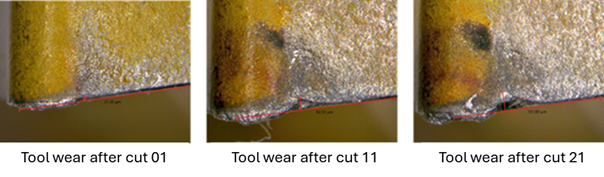
- Repeat steps 2–3; after cuts 1, 6, 11, 16, 21, and 26, remove the insert to measure flank wear.
- After the 26th cut, remove the cutting insert.
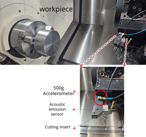
Figure 2 presents representative tool-wear measurements after the 1st, 11th, and 21st cuts of the same insert.
Data Overview
The dataset comprises face-cutting experiments on a DMG Mori NTX2500 machining stainless-steel cylindrical workpieces. An accelerometer and an acoustic emission (AE) sensor are mounted on the tool holder (see Figure 1). Each cutting insert performs 26 sequential cuts at a depth of 0.5 mm, with flank wear measured at selected intervals.
Sensors & Sampling
- Sensors: Tri-axial accelerometer (X/Y/Z in g) and AE RMS (V)
- Sampling rate: 25,600 Hz for both accelerometer and AE
- Axes mapping: X – neutral axis; Y – feed axis; Z – cutting axis
- Sensor CSV columns: Sample, Date/Time, Acceleration X (g), Acceleration Y (g), Acceleration Z (g), AE (V)
Controller (Process) Data
Per-cut controller logs are provided as CSV with the following 23 channels:
timestamp, progName, progStatus, feedrate,
mainSpndLoad, mainSpndSpd, mainSpndStatus,
toolSpndLoad, toolSpndSpd, toolSpndStatus,
X_load, Y_load, Z_load, A_load, B_load,
coolStatus, operMode, cut_no,
start_cut, end_cut, step_no, start_step, end_step.
Use start_cut and end_cut timestamps to slice the sensor records and extract the window for the current cut.
Similarly, start_step and end_step enable finer, step-level windows to zoom into sensor performance on a per-step basis.
Target Variable
- Target: Flank wear (depth of wear) of the cutting insert
- Label availability: Measured after cuts 1, 6, 11, 16, 21, 26 (see split-specific details in Training / Evaluation)
File Organization & Naming
- Controller files:
Controller_Data/<set>/Cut_01.csv…Cut_26.csv - Sensor bundles:
Sensor_Data/<set>/Part_01_1_1.zip,Part_02_2_6.zip,Part_03_7_11.zip,Part_04_12_16.zip,Part_05_17_21.zip,Part_06_22_26.zip(each ZIP contains the CSV(s) covering the indicated cut range) - Cut indexing: 1-based (
Cut_01…Cut_26) - Sets: Use
trainset_XXandevalset_XXas applicable; see the dedicated sections for split rules
Time & Synchronization
- Timestamps: Controller CSVs include a timestamp column; sensor CSVs include a Date/Time column and a Sample index
- Alignment: Use timestamps (or known sampling rate with Sample index) to align controller and sensor data per cut
Quick Start: Load Data with data_loader_trainset.py
from data_loader import DataLoader

# Root folders for controller and sensor data (works for both training and evaluation sets)
loader = DataLoader("Controller_Data", "Sensor_Data")

# Example: load controller + sensor for dataset #1, Cut #5
controller_df = loader.get_controller_data(1, 5)
sensor_df = loader.get_sensor_data(1, 5)

print("Controller shape:", getattr(controller_df, "shape", None))
print("Sensor shape:", getattr(sensor_df, "shape", None))
Split-specific visibility and labels are detailed in the Training Dataset and Evaluation Dataset sections.
Training Dataset
How it differs from the Evaluation set:
- Scope: 6 datasets (
trainset_01…trainset_06). - Visibility: Controller and sensor files for all 26 cuts are available.
- Labels: Flank wear after every cut (1–26) is provided.
- Intended use: Model development, ablation, and cross-validation (not used for official scoring).
- Formats: Per-cut controller CSVs; sensor data packaged per part/range in ZIPs (see Data Overview for channel list).
File Structure:
Training_Dataset/
├─ Controller_Data/
│  ├─ trainset_01/
│  │  ├─ Cut_01.csv
│  │  ├─ ...
│  │  └─ Cut_26.csv
│  │
│  ├─ .../
│  │
│  └─ trainset_06/
│     ├─ Cut_01.csv
│     ├─ …
│     └─ Cut_26.csv
│
├─ Sensor_Data/
│  ├─ trainset_01/
│  │  ├── Part_01_1_1.zip
│  │  │   └── accelerometer_data_1_1.csv
│  │  ├── Part_02_2_6.zip
│  │  │   └── accelerometer_data_2_6.csv
│  │  ├── Part_03_7_11.zip
│  │  │   └── accelerometer_data_7_11.csv
│  │  ├── Part_04_12_16.zip
│  │  │   └── accelerometer_data_12_16.csv
│  │  ├── Part_05_17_21.zip
│  │  │   └── accelerometer_data_17_21.csv
│  │  └── Part_06_22_26.zip
│  │      └── accelerometer_data_22_26.csv
│  │
│  ├─ .../
│  │
│  └─ trainset_06/
│     ├── Part_01_1_1.zip
│     │   └── accelerometer_data_1_1.csv
│     ├── Part_02_2_6.zip
│     │   └── accelerometer_data_2_6.csv
│     ├── Part_03_7_11.zip
│     │   └── accelerometer_data_7_11.csv
│     ├── Part_04_12_16.zip
│     │   └── accelerometer_data_12_16.csv
│     ├── Part_05_17_21.zip
│     │   └── accelerometer_data_17_21.csv
│     └── Part_06_22_26.zip
│         └── accelerometer_data_22_26.csv
│
│
└─ trainset_toolwear_measurement.csv
Evaluation Dataset
How it differs from the Training set:
- Scope: 3 datasets (
evalset_01…evalset_03). - Visibility: By default, only the earliest cut’s files are downloadable; subsequent cuts are hidden for scoring.
- Labels: Only the first available cut has a wear label; participants must predict the remaining cuts for each insert.
- Submission: Upload a Docker image to the PHM-AP Data Challenge Portal; the Portal executes your container and reads predictions for leaderboard scoring.
- Limits: Max 2 submissions per team per day (see Submission section for details).
File Structure:
*Only Cut_01 data is available for participant download; the remaining cuts are reserved for performance evaluation.
Evaluation_Dataset/
├─ Controller_Data/
│  ├─ evalset_01/
│  │  ├─ Cut_01.csv
│  │  ├─ ...
│  │  └─ Cut_26.csv
│  │
│  ├─ evalset_02/
│  │  ├─ Cut_02.csv  <-- no Cut_01 data, start from Cut_02
│  │  ├─ ...
│  │  └─ Cut_26.csv
│  │
│  └─ evalset_03/
│     ├─ Cut_01.csv
│     ├─ …
│     └─ Cut_26.csv
│
├─ Sensor_Data/
│  ├─ evalset_01/
│  │  ├── Part_01_1_1.zip
│  │  │   └── accelerometer_data_1_1.csv
│  │  ├── Part_02_2_6.zip
│  │  │   └── accelerometer_data_2_6.csv
│  │  ├── Part_03_7_11.zip
│  │  │   └── accelerometer_data_7_11.csv
│  │  ├── Part_04_12_16.zip
│  │  │   └── accelerometer_data_12_16.csv
│  │  ├── Part_05_17_21.zip
│  │  │   └── accelerometer_data_17_21.csv
│  │  └── Part_06_22_26.zip
│  │      └── accelerometer_data_22_26.csv
│  │
│  ├─ .../
│  │
│  └─ evalset_03/
│     ├── Part_01_1_1.zip
│     │   └── accelerometer_data_1_1.csv
│     ├── Part_02_2_6.zip
│     │   └── accelerometer_data_2_6.csv
│     ├── Part_03_7_11.zip
│     │   └── accelerometer_data_7_11.csv
│     ├── Part_04_12_16.zip
│     │   └── accelerometer_data_12_16.csv
│     ├── Part_05_17_21.zip
│     │   └── accelerometer_data_17_21.csv
│     └── Part_06_22_26.zip
│         └── accelerometer_data_22_26.csv
│
├─ data_loader.py
│
└─ evalset_toolwear_measurement.csv
Submissions
The PHM-AP 2025 Data Challenge Portal is the official channel for automated scoring on the Evaluation Dataset. Each team creates an account and uploads a Docker image for evaluation (email address is used as the login username).
- What to upload: A Docker image exported with
docker save(e.g.,docker save yourimage:tag -o image.taror gzip-compressedimage.tar.gz). - How it runs: Your container must run non-interactively and finish by itself (no manual input). The algorithm should complete within 1 hour; otherwise the procedure will be terminated automatically. Each team can run one task at a time.
- Read inputs from:
/tcdata(mounted read-only; containsController_Data,Sensor_Data, and the provideddata_loader.py). - Write outputs to:
/work/result.csv(mounted write-only; the Portal collects this file for scoring). - Result file: Save a single CSV named
result.csvto/work/. Follow the format defined in the Docker Guideline section. - Entry command: Provide an automatic entrypoint (e.g.,
CMD ["sh","run.sh"]). Avoid interactive shells. - Daily limit: Maximum 2 submissions per team per day.
- Batch schedule: Submissions are executed nightly starting 00:00 SGT (UTC+8); the leaderboard updates by 08:00 SGT.
- Hardware (Portal host): EC2
t3.large(2 vCPU, 8 GiB RAM) for fairness and reproducibility. - Network: Containers run offline (no internet access).
Notes: Use absolute paths where possible (e.g., /tcdata, /work).
For dataset visibility rules and file structures, see the Training Dataset and Evaluation Dataset sections.
Scoring
- Final ranking based on hidden Evaluation Dataset
- Each submission will be evaluated according to model prediction accuracy, measured by the following metrics: RMSE, MAPE and R²
- The overall ranking will be determined based on sub-ranks from each scoring metric (RMSE, MAPE, and R²). For each dataset, participants are ranked separately by RMSE, MAPE, and R². These sub-ranks are then summed (or averaged) to obtain an overall score, and participants are ordered accordingly to generate the final ranking.
Example:
| Team | RMSE Rank | MAPE Rank | R² Rank | Overall Rnk Basis | Final Overall Rank |
|---|---|---|---|---|---|
| A | 1 | 2 | 3 | 1+2+3=6 | 2nd |
| B | 2 | 1 | 1 | 2+1+1=4 | 1st |
| C | 3 | 3 | 2 | 3+3+2=8 | 3rd |
*If two or more teams have the same total sub-rank, ties will be broken in the following order: (1) lower RMSE, (2) lower MAPE, (3) higher R².
Datasets
Download the released datasets from Google Drive:
| Dataset | Download |
|---|---|
| Training Dataset (Training_Dataset.zip) | Google Drive Link |
| Evaluation Dataset (Evaluation_Dataset.zip) | Google Drive Link |
Leaderboard (Final Results)
This leaderboard reflects the final verified results after portal shutdown.
| Rank | Team Name | RMSE | MAPE (%) | R² |
|---|---|---|---|---|
| 1 | lone warrior | 10.052 | 7.878 | 0.904 |
| 2 | MIRIA | 10.417 | 9.004 | 0.897 |
| 3 | LAX | 10.644 | 8.041 | 0.892 |
| 4 | GSI-MACS | 11.486 | 8.518 | 0.875 |
| 5 | JNS Team | 11.461 | 9.508 | 0.875 |
| 6 | AION Nexus | 13.530 | 10.080 | 0.826 |
| 7 | WornOut | 14.484 | 13.671 | 0.801 |
| 8 | Chaos | 14.499 | 13.351 | 0.800 |
| 9 | PrognosTech | 14.603 | 12.709 | 0.797 |
| 10 | ENPHM | 15.338 | 14.880 | 0.776 |
| 11 | XJTU | 15.449 | 14.538 | 0.773 |
| 12 | saraca | 16.469 | 15.886 | 0.742 |
| 13 | ds | 16.824 | 16.228 | 0.731 |
| 14 | ProGENy | 18.055 | 15.589 | 0.690 |
| 15 | NewbieAI | 18.373 | 17.178 | 0.679 |
| 16 | mnm3 | 21.111 | 19.581 | 0.576 |
| 17 | Ubix | 23.469 | 19.460 | 0.476 |
| 18 | ENAS_PHM_TEAM | 26.789 | 22.758 | 0.318 |
| 19 | YY | 29.068 | 26.933 | 0.197 |
| 20 | Aegis | 32.292 | 31.291 | 0.008 |
| 21 | SJTUME | 40.333 | 26.331 | -0.547 |
| 22 | Spartans | 42.554 | 34.498 | -0.722 |
| 23 | Kunlong_Huang | 59.454 | 50.806 | -2.361 |
| 24 | IKERLAN-UPC | 59.593 | 56.401 | -2.377 |
| 25 | kfl372 | 68.183 | 57.764 | -3.421 |
| 26 | OVO | 396.204 | 351.670 | -148.276 |
| 27 | keepgoing | 468.396 | 417.494 | -207.630 |
| 28 | LDM | 548.521 | 487.306 | -285.113 |
| 29 | toocool | 622.787 | 554.761 | -367.833 |
| 30 | Avish | 1005.962 | 846.917 | -961.307 |
| 31 | hehekk | 1372.563 | 1066.264 | -1790.494 |
| 32 | CDTC | 1383.216 | 1229.769 | -1818.409 |
| 33 | CQU_1 | 1462.818 | 1175.724 | -2033.844 |
| 34 | DonRyu | 1531.774 | 1139.187 | -2230.208 |
Docker Image Guideline
All participant solutions must be submitted as Docker images via the Data Challenge Portal (CPU-only environment). Each team may submit up to two Docker images per day. Submissions are executed automatically at 00:00 midnight, and leaderboard results are released by 08:00 AM daily. The total inference runtime for each image must not exceed one hour.
1. Computing Resources
- Instance type: AWS EC2 t3.small
- CPU: 2 vCPU
- Memory: 4 GiB
- GPU: Not available (CPU-only)
2. Docker Image Requirements
- Include a
run.shscript in the root directory. It will be used as the container entry point. - The
run.shscript must:- Load the pre-trained model and dependencies.
- Read all input data from the
/tcdatafolder (read-only mount). - Generate predictions and save them to
/work/result.csv.
- Ensure the image runs correctly with:
docker run -v $(pwd)/tcdata:/tcdata -v $(pwd)/work:/work your_image sh run.sh
Expected Output Format
Your result.csv must be saved in /work/ and follow the format below:
| set_num | cut_num | pred |
|---|---|---|
| evalset_01 | 2 | 5 |
| evalset_01 | 3 | 2 |
| evalset_02 | 2 | 3 |
| evalset_03 | 26 | 1.4 |
Where set_num ∈ {evalset_01, evalset_02, evalset_03} and cut_num ∈ [2, 26].
The evaluation system automatically collects and validates /work/result.csv.
Incorrect file naming or missing results will result in a failed submission.
3. Dataset Mounting Structure
The hidden evaluation dataset is automatically mounted at /tcdata (read-only).
The structure is as follows:
tcdata/
├─ Controller_Data/
│  ├─ evalset_01/
│  ├─ evalset_02/
│  └─ evalset_03/
└─ Sensor_Data/
   ├─ evalset_01/
   ├─ evalset_02/
   └─ evalset_03/
4. Recommended Best Practices
- Use
python:3.9-slimorpython:3.x-slimas the base image. - Declare dependencies in
requirements.txt. - Use absolute paths (
/tcdata,/work) instead of relative paths. - Keep image size below 3 GB for reliable uploads and runtime.
- Print progress messages to
stdoutfor debugging. - Never write to
/tcdata(it is read-only).
5. Example File Layout
project/
├── Dockerfile
├── run.sh
├── main.py
├── requirements.txt
├── model/
│   └── xgb_model.pkl
└── lib/
    ├── data_loader.py
    └── feature_engineering.py
6. Docker Creation Reference
-
Create a Dockerfile:
FROM python:3.13-slim WORKDIR /workspace COPY requirements.txt . RUN pip install --no-cache-dir -r requirements.txt COPY lib/ lib/ COPY model/ model/ COPY main.py . COPY run.sh . RUN sed -i 's/\r$//' run.sh && chmod +x run.sh CMD ["sh", "run.sh"] -
Write run.sh:
#!/bin/sh
echo "Starting PHM2025 docker image run..."
python main.py

if [ -f /work/result.csv ]; then
    echo "Results saved at /work/result.csv"
else
    echo "result.csv not found, check logs."
    exit 1
fi
Always save predictions to
/work/result.csv. -
Write main.py:
import os
import joblib
import pandas as pd
import numpy as np
from lib.data_loader import DataLoader
from lib.feature_engineering import get_features

def main():
    """
    Run evaluation on all controller and sensor datasets,
    extract features, apply the trained model, and save predictions.

    Output:
    - result.csv saved to /work directory
    """

    controller_path = '/tcdata/Controller_Data'
    sensor_path = '/tcdata/Sensor_Data'
    output_path = '/work/result.csv'
    model_path = 'model/xgb_model.pkl'

    evalset_list = [1, 2, 3]
    cut_list = list(range(2, 27))

    loader = DataLoader(controller_path, sensor_path)
    records, features = [], []

    for set_no in evalset_list:
        for cut_no in cut_list:
            print(f'Processing Cut {cut_no} in Set {set_no}...')
            controller_df = loader.get_controller_data(set_no, cut_no)
            sensor_df = loader.get_sensor_data(set_no, cut_no)
            tmp_features = get_features(controller_df, sensor_df)

            records.append([f'evalset_{set_no:02d}', cut_no])
            features.append(tmp_features)

    result_df = pd.DataFrame(records, columns=['set_num', 'cut_num'])
    loaded_model = joblib.load(model_path)

    features = np.array(features, dtype=float)
    pred = loaded_model.predict(features)

    result_df['pred'] = pred
    result_df.to_csv(output_path, index=False)
    print(f"Results saved to {output_path}")

if __name__ == '__main__':
    main()
This template demonstrates how to iterate through evaluation sets, process data, and generate predictions for scoring.
-
Build and save your Docker image:
docker build -t phm-sample .
docker save -o phm-sample.tar phm-sample
Upload the
.tarfile through the Data Challenge Portal.
Tips
- Test locally using:
docker run --rm -v $(pwd)/tcdata:/tcdata -v $(pwd)/work:/work phm-sample - Ensure
run.shuses Unix line endings (LF) if edited on Windows. - Remove unnecessary packages and caches to minimize image size.
Mounted Folders Inside Docker
/tcdata→ Input data (read-only)/work→ Output folder (write-only, must containresult.csv)
Common Troubleshooting
- “result.csv not found” → Ensure output path is
/work/result.csv. - Permission denied → Add
chmod +x run.shin Dockerfile. - Wrong file paths → Always use absolute paths, not relative ones.
- Windows CRLF issue → Fix with
sed -i 's/\r$//' run.sh. - Large image → Use slim base images and delete cache files.
Data Challenge Portal
This page provides information about the Data Challenge Portal status.
Portal Shutdown Notice
The PHMAP2025 Data Challenge Portal has been permanently shut down following the completion of the competition. Docker submissions, automated scoring, and leaderboard updates are no longer available.
The final leaderboard is now published on this website and will remain as the official permanent record of the competition results.
We thank all teams for their participation and contributions to the challenge.
For any post-competition enquiries, please contact the PHMAP2025 committee.